Quickstart Guide¶

Removing Duplicates¶

To get the duplicates in a directory with structures, you can run something like

from structure_comp.remove_duplicates import RemoveDuplicates

rd_rmsd_graph = RemoveDuplicates.from_folder(
    '/home/kevin/structure_source/csd_mofs_rewritten/', method='rmsd_graph')

rd_rmsd_graph.run_filtering()

The filenames and the number of duplicates are saved as attributes of the RemoveDuplicates object.

Warning

Large databases (e.g. CCSD MOF subset) can require a large a amount of temporary hard drive (“swap”) space which we use to store the Niggli reduced structures. As the main routine runs in a contextmanager, the temporary files will be deleted even if the program runs into an error. If you use cached=True we will not write temporary files but keep everything in memory. This is of course not feasible for large database.

We already use KDTrees and spare matrices where possible to reduce the memory requirements.

Getting Statistics¶

Measuring the diversity of a dataset¶

If you have properties – great, use those! With you don’t have any, calculate some using some package like zeo++ or matminer. If you really want to compare structures, you can use the DistStatistic class. Using the randomized RMSD is decently quick, constructing structure graphs can take some time and probably does not lead to more insight:

from structure_comp.comparators import DistStatistic
core_cof_path = '/home/kevin/structure_source/Core_Cof/'

# core cof statistics
core_cof_statistics = DistStatistic.from_folder(core_cof_path, extension='cif')
randomized_rmsd_cc = core_cof_statistics.randomized_rmsd()
randomized_jaccard_cc = core_cof_statistics.randomized_graphs(iterations=100)

Then, it might be interesting to plot the resulting list as e.g. a violinplot to see whether the distribution is uniform (which would be surprising) or which RMSDs are most common as well as (what is probably most interesting) what is the width of the distribution. A example is shown in the Figure below.

Comparing two property distributions¶

If you have two dataframes of properties and you want to find out if they come from the same distribution the DistComparison class is the one you might want to use.

Under the hood, it runs different statistical tests feature by feature and some also over the complete dataset and then returns a dictionary with the test statistics.

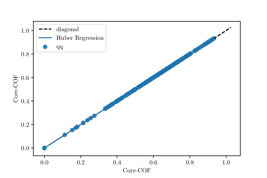
QQ-plot¶

Something really useful is to do a QQ-test. By default, we will plot the result but also give you some metrics like the deviation of the slope of Huber regression trough the qq-plot from the diagonal. If the distributions are identical, you should see something like

QQ-plot for the void fractions of the structures in the Core-COF datset. [TLYZ17].¶

Whereas, if the value of the property is consistently lower for one dataset, we would expect something like

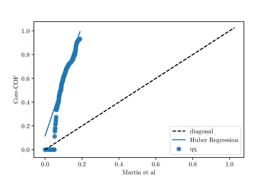
QQ-plot for the void fractions of the structures in the Core-COF datset and the hypothetical COF dataset of Martin et al.¶

To run the QQ-test, you only need something like the following lines

void_fraction_martin_cc = DistComparison(property_list_1=df_martin['voidfraction'].values,
                     property_list_2=df_cc['voidfraction'].values)

void_fraction_martin_cc.qq_test()

In our results dictionary, we would find 'deviation_from_ideal_diagonal': -3.6 which indicates that the Huber regression is much steeper than the diagonal.

Statistical tests¶

Besides the QQ-test/plot you can also choose to run a variety of statistical tests on the dataset. If you provide multiple feature columns, we will run the tests column-wise and some of them globally.

A nice overview about some statistical tests can be found some Jupyter notebooks by Eric Schles.

To run the statistical tests, you can use some code snippet like the following

comparator = DistComparison(property_list_1=df0, property_list_2=df1)
result_dict = comparator.properties_test()

where df0 and df1 are the two property dataframes (they need to have the same number and order of columns, if you provide a dataframe, we will use the column names as keys in the output dictionary).

Finding out if a structure is different from a distribution¶

In this case you have the following possibilities:

you can do a property-based comparison
you can do a structure based comparison, guided by properties
you can do a random structure based comparison

Sampling¶

The sampler object works on dataframes, since this interfaces smoothly with featurization packages like matminer. So far, a greedy and a clustering-based farthest point sampling have been implemented.

To start sampling you have to initialize a sampler object with dataframe, columns, the name of the identifier column and the number of samples you want to have:

from structure_comp.sampling import Sampler
import pandas as pd
zeolite_df = pd.read_csv('zeolite_pore_properties.csv')
columns = ['ASA_m^2/g', 'Density', 'Largest_free_sphere',
     'Number_of_channels', 'Number_of_pockets', 'Pocket_surface_area_A^2']
zeolite_sampler = Sampler(zeolite_df, columns=columns, k=9)

# use the knn-based sampler
zeolite_samples = zeolite_sampler.get_farthest_point_samples()

# or use the greedy sampler
zeolite_sampler.greedy_farthest_point_samples()

If you want to visualize the samples, you can call the inspect_sample function on the sampler object:

zeolite_sampler = inspect_sample()

If you work in a Jupyter Notebook, don’t forget to call

%matplotlib inline

Cleaning Structures¶

Rewriting a `.cif` file¶

Most commonly we use the following function call to “clean” a .cif file

from structure_comp.cleaner import Cleaner

cleaner_object = Cleaner.from_folder('/home/kevin/structure_source/csd_mofs/', '/home/kevin/structure_source/csd_mofs_rewritten')
cleaner_object.rewrite_all_cifs()

You will find a new directory with structures that:

have “safe” filenames
have no experimental details in the cif files
are set to P1 symmetry
have a _atom_site_label column that is equal to _atom_site_type_symbol which we found to work well with RASPA
by default, we will also remove all disorder groups except . and *
optionally you can also remove duplicates (atoms closer 0.1 sAngstom) using a ASE routine.

If you input files have a _atom_site_charge column, you wil also find it in the output file.

Note

You also have the option to symmetrization routines by setting clean_symmetry to a float which is the tolerance for the symmetrization step.

Removing unbound solvent¶

Warning

Note that this routine is slow for large structures as it has to construct the structure graph.

Remove disorder¶

For removal of disorder, we implemented two algorithms of different complexities. One performs hierachical clustering on the atomic coordinates and then merges the clashing sites of same elements.

To more naive version, simply build a distance matrix (a KDTree for efficiency reasons) and then merges the the clashing sites with following priorities: * if the elements are the same, the first site remains * if the elements are different, the heavier element remains

A code that is conservative (first uses the checker and then fixes the issues separately) could look as follows

::

from structure_comp.utils import read_robust_pymatgen from pathlib import Path

for structure in clashing_structures:: s = read_robust_pymatgen(structure) name = Path(structure).name s_cleaned = Cleaner.remove_disorder(s, 0.9) s_cleaned.to(filename=os.path.join(‘unclashed’, name))

Checking structures¶

To run a large variety of checks on a structural database you can use something like

from structure_comp.checker import Checker
from glob import glob
import pandas as pd

checker_structures = glob('*/*.cif')
checker_object = Checker(checker_structures)

problems_df = checker_object.run_flagging()
problems_df.head()